This exercise came out of a series of lectures given for the Topological QFTs reading group. Really the lectures began as a way to catch up on elementary knot theory so that the group could further understand the work of Vaughan Jones. This post is not meant to be tremendously theoretical, but meant to serve as a gentle reminder about how one does these sorts of computations.
Define. A knot is a closed curve seen as a subset $K \subset S^3$ which
should be interpreted as $\mathbb{R}$ plus a point at infinity.
There are reasons for why the point at infinity is useful (although it is not
relevant to the current task) and I believe containing the knot in $S^3$ is done
so that we can fit the whole knot in a compact space. There are some operations
on knots, but all we need here is to understand that knots can be linked. A
link $L$ is a collection of non-intersecting knots that are “linked” together. A
good example of this is the Borromean link
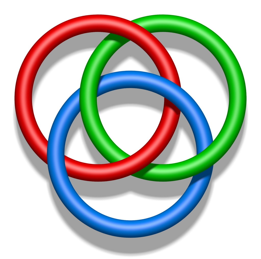
Each ring here (which is really just a circle) is called an “unknot”. Observe
that the removal of any unknot from the picture would totally undo the link.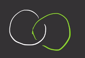
Hopf link
A subtle detail of my drawing of the Hopf link: at the crossing there is
one completely solid line intersection a “broken” line. The broken line is to be
interpreted as the string which passes under the other string in the crossing.
One goal of knot theory is to classify knots. One way we can do this is to
capture a knot with algebraic information. In the case of the Jones polynomial
one must use a Laurent polynomial. First I’ll start with a more general
polynomial for knots known as the Kauffman bracket which is most easily defined inductively. For any link $L$ the Kauffman bracket $\langle L \rangle$ is
- $\langle L \rangle = 1$ if $L$ is the unknot.
- $\langle \times \rangle = A \langle || \rangle + A^{-1} \langle = \rangle$
- $\langle U \sqcup L = (-A^2 - A^{-2})\langle L \rangle$ (where $U$ is the
unknot and $L$ is some link)
Rule 2 will require further explanation. The symbols $\times$, $||$, and $=$ are
meant to be seen as physical string. $\times$ implies there is a crossing, $||$
implies the strings are vertical and parallel whereas $=$ implies the strings
are horizontal and parallel. The idea is to “smooth” or reduce knot crossings
into the sum of these two components.
So we can decompose the Hopf link using a recursive approach in a sort of tree
structure such as:
R_{\beta}e^{i \varphi_\beta}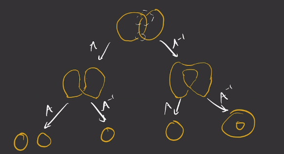
The diagram starts with the Hopf link and then we apply a single smoothing to a single crossing. I label the edges of my graph by the coefficient attached to the smoothing given by rule 2. The bottom middle two nodes of the tree are just unknots, and so their Kauffman brackets
are constant 1. Now the bottom left and bottom right nodes are regular isotopies of another (meaning one can be transformed to the other by Reidemeister move’s of type II and III). All that remains is to compute the Kauffman bracket of the double unkot.
By rule (1) a single unknot $U$ has bracket 1. By rule 3 $\langle U \sqcup U \rangle = (-A^2 - A^{-2})\langle U \rangle = (-A^2 - A^{-2})$. Meaning if we sum our components we get $$A^2(-A^2-A^{-2})+1+1+A^{-2}(-A^2 -A^{-2}) = -A^4 - A^{-4}$$
Something else you could do is start with a sum of all possible smoothings.
Suppose the unknot’s polynomial is $-A^2 - A^{-2}$ then instead of a recursive
tree you could have a list of all possible smoothings (where we smooth all
crossings at the same time)

Notice the sum here is $(A^2 + A^{-2})(A^4 + A^{-4})$ which has an additional
factor on our answer from the recursive approach. Remembering that we “scaled”
the unknots polynomial, we can renormalize by dividing out $(-A^2 - A^{-2})$
Now if $A^4 = t$ this is Jones polynomial of the Hopf link (in fact
orienting the link and multiplying the bracket by a factor $A^{-3wr(L)}$ will
get you to the Jones polynomial).
A question that I spent some time thinking about is how to motivate $-A^2 - A^{-2}$ as the choice for the unknot’s bracket. This expression is obviously not very random. For one, it has the nice property that $\langle \bigsqcup U_n \rangle = (-A^2 - A^{-2})^n$ where $U_n$ is a length $n$ sequence of unknots. It also happens to show up in the invariance of the Kauffman bracket under the Reidemeister type II move which Sanchayan Dutta recently wrote about. Namely, it is the constant $\delta$.